Debt Schedule PMT IPMT If Formulas

What is Debt Schedule PMT IPMT If Formulas?

A debt schedule utilizes formulas like PMT, IPMT, and IF to construct a detailed table outlining periodic payments towards a loan.

The PMT, PPMT, and IPMT functions are three financial functions widely used in Excel. These three functions are related to each other.  If someone is seeking to borrow money, they have numerous avenues to explore, which will depend on various factors. 

Key considerations include the interest rate, whether it is compounded monthly or annually, and the total interest needed over the original loan amount. All these questions are answered using a combination of Excel's PMT, PPMT, and IPMT functions.

PMT Function in Excel

The term PMT refers to a payment made in each period. The PMT function in Excel returns the total payment (principal amount + interest money) that has to be made while repaying a loan or the total amount we get while we receive returns on investment.

The syntax used for the PMT formula in Excel is as follows:

=PMT(rate, nper, pv, [fv], [type]) 

The terms in parentheses are called the arguments of the function. 

Here, 

• rate is the interest rate for each period.
• per is the number of periods for which the principal amount is demanded. 
• nper is the total number of periods. 
• pv is the present value of the loan or investment. 
• fv refers to the future value of the loan or investment. 
• type is an integer argument whose value is 
  • 1 if the payments are made at the start of each period
  • 0 if the payments are made at the end of each period

The PMT function does not require the per argument because:

Total Payment (PMT)= Principal Amount (PPMT) + Interest Amount (IPMT)

Examples of PMT Function in Excel

Having looked at the basic definition and meaning of the PMT function in Excel, let us now look at some examples showing the practical application and usage of the PMT function:

Example 1

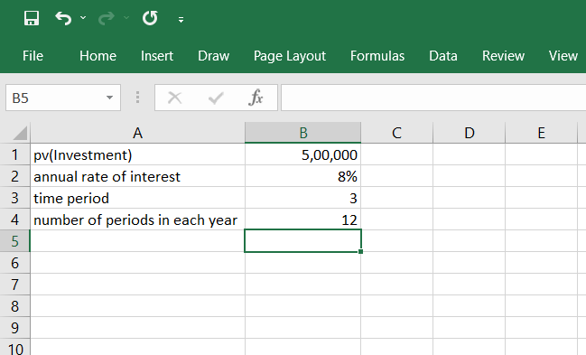
Assuming an investment of rupees 5,00,000 made by a business in the real estate sector at a constant annual rate of interest of 8% for three years, let's calculate the total monthly payment using the PMT function.

To calculate the total monthly payment, we use the following formula:

=PMT(B2/B4, B3*B4, -B1)

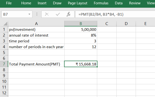
Using the PMT function, we get the total installment amount for each period to be 15,668.18.

Here, the annual interest rate is 8%, with 12 periods in a year. So, the periodic interest rate becomes (8/12)% or B2/B3. The total number of periods (nper) is the total number of years multiplied by the number of periods each year. Therefore, nper is B3*B4.

Example 2

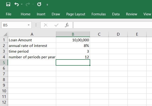
Suppose Mr. Johnson took a loan of rupees 10,00,000 from a bank at an annual interest rate of 8% for three years, with 12 periods in a year.

To get the amount, Mr. Johnson has to pay at the end of each period, we use the following PMT formula:

= -PMT(B2/B4, B3*B4, B1)

Here, we use B1 instead of -B1 in the formula for the PMT function, unlike example 1, because in this case, there is a cash outflow, which means Mr. Johnson has to give away money to repay the loan.

Therefore, this formula does not need a negative sign because the cash outflow is already accounted for.

In example 1, the firm received money(cash inflow) as investment returns. Hence, an extra negative sign comes whenever there is a cash outflow.

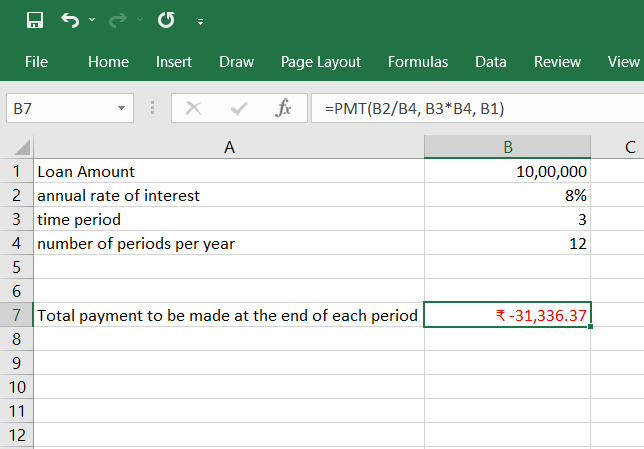
Hence, the PMT function returns the periodic payment debited for each period as -31,336.37. Here, the negative sign indicates that there has been a cash outflow, and the amount paid at the end of each period is rupees 31,336.37.

PPMT Function in Excel

The term PPMT refers to the principal amount paid in each period when taking a loan. The PPMT function in Excel isolates and determines the principal amount from the total payment to be made at the end or beginning of a period. 

If a person or firm has taken a loan, the interest amount will decrease as more periods pass, whereas the principal amount to be paid increases to settle the loan. The syntax used for the PPMT function in Excel is:

=PPMT(rate, per, nper, pv, [fv], [type])

All the function arguments are explained above.

Here: 

• nper should always be a positive number as it represents the total number of periods

• per argument must lie between 1 and nper.

Generally, the PPMT function is not preferred in creating a debt schedule as we can directly calculate the principal amount for a period(PPMT) as the difference between the total payment(PMT) and the interest amount(IPMT). 

For creating a debt schedule, the preferred approach involves using the PMT function, IPMT function, and another function in Excel called the IF function. These functions combined provide the necessary calculations for generating a comprehensive debt schedule.

Examples of PPMT Function in Excel

Some practical applications of the PPMT function in Excel can now be explored after understanding what it means.

Example 1

Considering the same scenario as example 1 for the PMT function, where a business invested rupees 5,00,000 at an annual interest rate of 8% for three years. 

To calculate the principal amount for the first period, we use the formula:

=PPMT(B2/B4, 1, B3*B4, -B1)

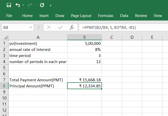
Using the PPMT function, we get the principal amount for the first period as 12,334.85. Here, the value of the function argument per is 1, as we need to calculate the principal amount for the first period. However,  fv and type have the default values(0).

Example 2

Considering the same scenario as example 2 for the PMT function, Mr. Johnson took out a loan of rupees 10,00,000 for 3 years. The annual interest rate for the loan was 8%.

We intend to calculate the principal amount of money Mr. Johnson would have to pay in the first three periods, which means the value of argument per is 1, 2, and 3, respectively. To calculate the principal amount paid in the first period, we can use the following formula:       

=PPMT($B$2/$B$4, A10, $B$3*$B$4, $B$1)

Similarly, we use cells A11 and A12 to calculate the principal amount in the second and third periods.

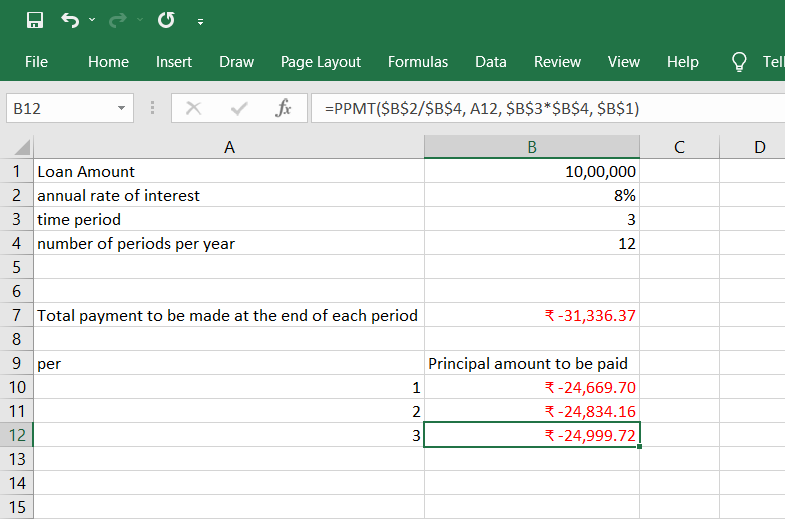
The PPMT function returns rupees 24,669.70 as the principal amount for the first period. Then, we use the fill-handle tool in Excel to get the principal amount for each subsequent period.

IF Function in Excel

As discussed above, the PPMT function could be more helpful in creating a debt schedule. So instead, we use the IF function as a useful tool when creating a debt schedule or performing other conditional calculations.

It determines if a given condition is true or false and returns corresponding values. The IF function has the following syntax:

=IF(logical_test, [value_if_true], [value_if_false])

Let's break down the components of the IF function:

1. logical_test: This is the condition that you want to evaluate. It can be a comparison between two values using operators such as greater than (>), less than (<), equal to (=), etc. The logical test determines if the condition is true or false.
2. value_if_true: This is the value that will be returned if the logical_test evaluates to true. It can be a number, text, cell reference, or another formula.
3. value_if_false: This is the value that will be returned if the logical_test evaluates to false. Like value_if_true, it can be any value or expression. The IF function allows users to make a logical comparison between two values.
   • It can also check for the equality of two strings/texts, but it cannot check whether one text is greater than or less than another string.

Examples of IF Function in Excel

Having seen what the IF function intends to do, let us now look at a few examples showing the applications of the IF function in Excel.

Example 1

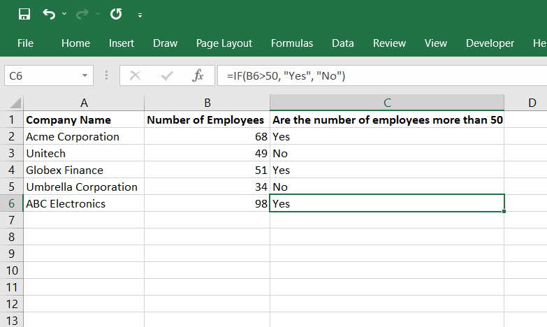
Let us consider the data in which we want to return yes if the number of employees in a hypothetical company listed in column B is greater than 50, or else we return no. Using the IF function, the formula would be:

=IF(B2>50, "Yes", "No")

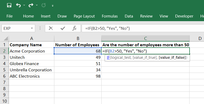
This formula checks the condition B2>50. If the number of employees is more than 50, which means the condition is True, it returns yes or no. The formula can be applied to all the cells in column C to get the corresponding results.

Similarly, we can also check for equality using the IF function. Let us see another example of the IF function.

Example 2

Let us consider the following data, showing the monthly earnings and expenditures of 5 people.

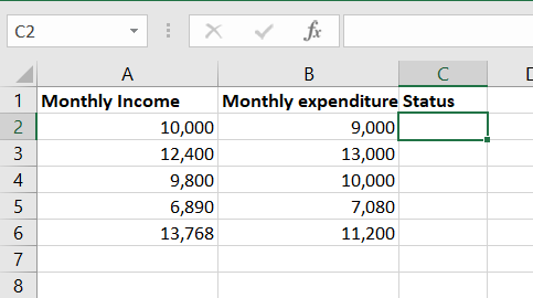
We need to check if the monthly expenditure is more than the monthly income and return overspending if it is True or else return normal spending for all five people. Using the IF function, the formula would be:

=IF(B2>A2, "Overspending", "Normal spending")

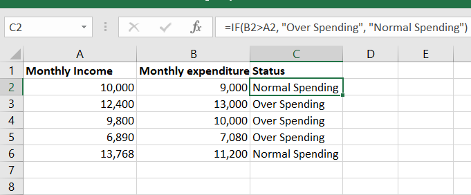
This formula checks if the monthly expenditure (column B) exceeds the monthly income (column A). If the condition is true (i.e., there is overspending), it returns "Overspending." Otherwise, it returns "Normal spending." 

In this way, we can use the IF function in Excel to check different conditions and return the desired value.

IPMT Function in Excel

The IPMT function is another financial function in Excel. The acronym IPMT refers to the amount of interest paid. The IPMT function in Excel returns the money to be paid as interest from the total payment transacted at the beginning or end of each period. 

When we take a loan, we return the interest with the principal amount. The syntax for the IPMT function in Excel is as follows:

=IPMT(rate, per, nper, pv, [fv], [type])

This formula calculates the interest amount based on the amount of loan due and the period. We can calculate the interest amount paid in any period using the IPMT function. 

In the above formula, the argument per gives the period number for which we are calculating the interest amount. The per always lies between 1 and nper (the total number of periods). 

All the function arguments are explained above in the discussion of the PMT function. In the following topic, we will explore examples demonstrating the practical applications of the IPMT function in Excel.

Examples of IPMT Function in Excel

The IPMT function in Excel is useful for calculating the interest amount paid in each loan period. We can apply it to practical examples by understanding its syntax and usage.

Example 1

Consider a business that invested rupees 5,00,000 at an annual interest rate of 8% for three years. To calculate the interest earned in the first period, we would use the following formula:

=IPMT(B2/B4, 1, B3*B4, -B1)

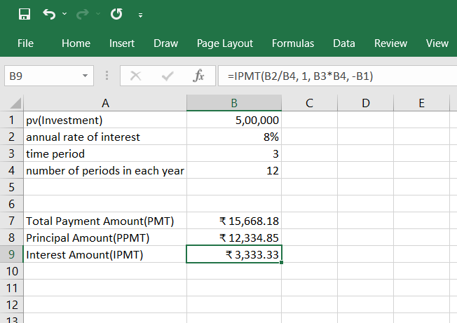
The formula returns the interest amount received by the firm for the first period to be rupees 3,333.33. As seen above, the total installment amount for each period is 15,668.18, and the principal amount for the first period is 12,334.85.

Hence, we can verify that:

Total Installment (15,668.18) = Principal Amount (12,334.85) + Interest Amount (3,333.33)

Example 2

Suppose Mr. Johnson took a loan of rupees 10,00,000 from a bank at an annual interest rate of 8% for three years.

We will now calculate the amount of money from the total payment, which is the interest, by using the IPMT function. We use the following formula to get the interest amount for the first period:

=IPMT($B$2/$B$4, A10, $B$3*$B$4, $B$1)

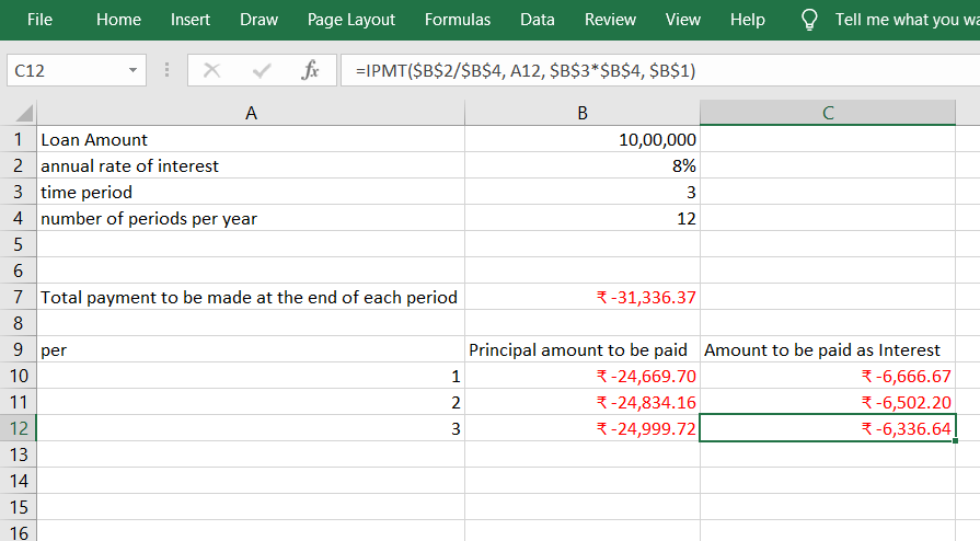
Consequently, we may use cells A11 and A12 as values of the argument per for calculating the interest amount in the second and third periods. 

As calculated above, the total payment for each period is 31,336.37(a negative sign indicating a cash outflow), and the principal amounts for the first three periods are 

1. 24,669.70 

2. 24,834.16

3. 24,999.72 

Hence, we can verify that: 

Total Payment Amount(PMT)= Principal Amount(PPMT) + Interest Amount(IPMT)

Similarly, we can calculate the principal and interest amount for each period. The payment calculated by PMT is constant for every period. In this case, the total number of periods is 36(as the loan is for three years and there are 12 periods in a year).

These examples demonstrate how the IPMT function can be applied to calculate interest amounts in different loan scenarios, allowing for accurate debt analysis and planning.

Creating a Debt Schedule Using the PMT, IPMT, and IF Functions

After learning about the different financial functions, we will create a debt schedule in Excel using PMT, IPMT, and the IF function. By following the steps outlined, you can construct a comprehensive debt schedule:

1. Assume debt details: Assume the debt to be rupees 50,000 at an annual interest rate of 6% for five years. The opening balance in the debt schedule is the loan amount of rupees 50,000.

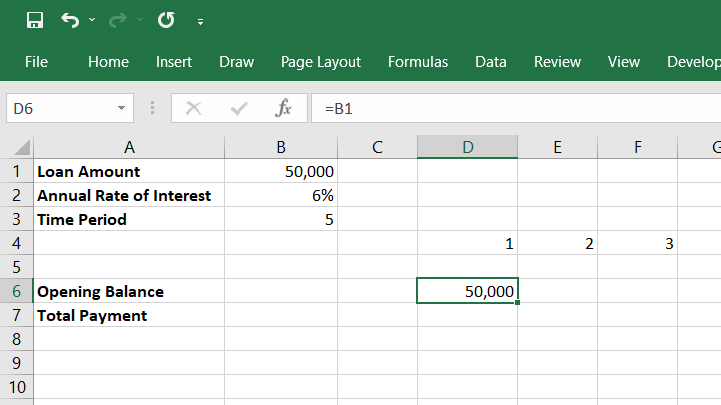
2. Set up the debt schedule: In cell B6, we write =B1, as shown above. Row 4 shows the period number. So, cell D4 represents the first period, and so on.

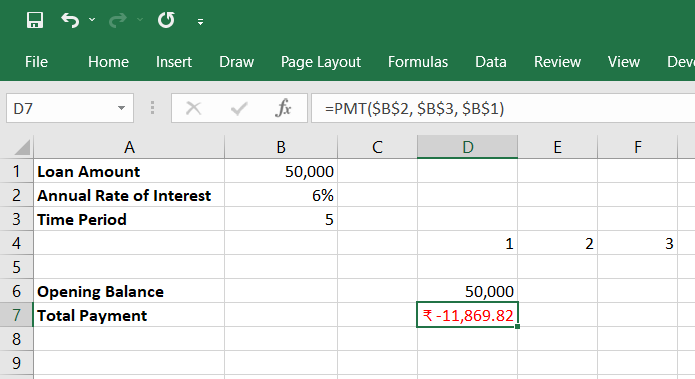
3. Calculate the total payment: Use the PMT function to calculate the total payment made in the first period

= PMT($B$2, $B$3, $B$1)

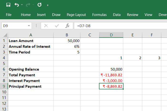
4. Calculate the interest payment: Use the IPMT formula to get the interest amount for the first period

= IPMT($B$2, D4, $B$3, $B$1)

5. Calculate the principal payment: The principal payment for the first period is the difference between the total payment and the interest payment in the first period, which can be calculated as D8-D7, as shown below. Doing this is the same as calculating PPMT.

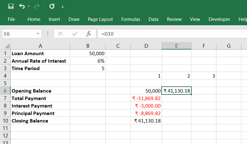
6. Calculate the closing balance: The closing balance in the debt schedule is the opening balance plus the principal amount, which can be calculated as D6+D9 for the first period. 

7. Determine the opening balance for the next period: The opening balance for the second period is the closing balance for period 1, so in cell E6, we write =D10 as shown below.

8. Copy the formulas: We can repeat the formulas used to calculate the opening balance, total payment, interest payment, principal payment, and closing balance in period 1 for all periods.

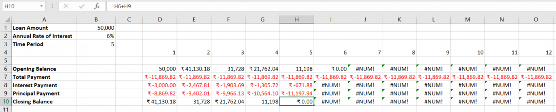
9. Handle error messages: Some error messages are displayed from period six onwards. The reason for these error messages is that the opening balance is 0. Hence, an error message #NUM! is displayed. We can clear all these errors by using the IF function.

To do so, in cell D7, we type:

=IF(D6>0, PMT($B$2, $B$3, $B$1), 0)

This formula means that if the opening balance is less than or equal to zero, the total payment amount would be 0, or it would show the amount calculated by the PMT formula.

10. Copy the IF function: Copy the above formula, select all cells from D7 to O7, and press Ctrl + R. This is the shortcut to fill right in Excel. Doing this pastes the above formula in all the selected cells, which means D7 to O7.

As shown above, the total payment in period 6 becomes 0 as the opening balance in period 6 is 0.

Similarly, in cell D8, we type:

=IF(D6>0, IPMT($B$2, D4, $B$3, $B$1), 0)

This formula is very similar to the previous one and means that if the opening balance is less than or equal to 0, the interest payment amount would be 0.

11. Remove error messages for interest payment: We again fill the above formula by copying the formula, selecting all cells from D8 to O8, and then pressing Ctrl + R. This pastes the above formula in all the selected cells from D8 to O8. Now, all the error messages are shown as 0.

12. Copy the IF function for interest payment: We can use the IF function to remove all the error messages and make our debt schedule look neater.

Here, we have obtained the debt schedule for the first 12 periods for the first year. However, using the above methods, we can easily calculate the opening balance, total payment, interest payment, principal payment, and closing balance for all periods and obtain the complete debt schedule using Excel's PMT, IPMT, and IF functions.

Researched and authored by Devang Shekhar | LinkedIn

Reviewed and edited by Parul Gupta | LinkedIn

Free Resources

To continue learning and advancing your career, check out these additional helpful WSO resources:

• Basic Excel Formulas

• HLOOKUP Function

• If Statement Between Two Numbers

• VLOOKUP

• XLOOKUP Function